Interface Reference · The Acoustics workspace

Acoustics Panels

The Acoustics workspace works as one instrument: you describe the scenario in Acoustics Setup (with the soundscape set on the Ambient Noise panel, which lives in the OCEAN group), and MuirWave shows the result in the Propagation plots and the Predicted Output card. This page walks every control on each panel and what the numbers mean.

$The Propagation panel computing: sound-speed profile on the left, ray fan refracting across range on the right, with the ACOUSTICS panel group lit in the rail.$

The ACOUSTICS group. Its tiles run down the rail — Acoustics Setup, Propagation, Output, Export. (Ambient Noise sits in the OCEAN group, just below Currents — it's a property of the water, and it feeds the acoustic noise term.) Shown: Propagation computing a complete scenario (SSP at left, ray fan at right; all four ACOUSTICS dots lit). Until you've set the four required parameters — Frequency, Source Level, Source Depth, Receiver Depth — the solver-driven panels instead show a checklist prompt (the deliberate no-defaults gate).

§01

How the panels fit together

Two panels are inputs — the knobs that define your scenario. Two are outputs — pictures and numbers the solver derives from those inputs. Everything flows left to right: set it, solve it, read it.

The Acoustics workspace, end to end. Acoustics Setup and Ambient Noise define the scenario; the map pins place it on the chart; the ray solver ties them together; the Propagation plots and Predicted Output card show what it means.

The four required parameters. The Propagation plots and the Predicted Output card don't compute from placeholder values. Until you've set Frequency, Source Level, Source Depth and Receiver Depth, those panels show a SCENARIO INCOMPLETE checklist instead of numbers. Fill the four in on Acoustics Setup and the results appear.

Source pin vs. probe. The solver-driven readouts (Predicted Output, the Ray Path field) are anchored to your source pin and target. The two "what's here?" readouts — the Ambient Noise spectrum and the SVP sound-speed curve — follow the probe, the movable inspection cursor on the map, so you can sample conditions anywhere without disturbing the scenario.

§02

Acoustics Setup

The scenario builder, in two groups: Source (what's making the sound) and Receiver (what's listening, and how). Every numbered row works the same way — tap the row to reveal a slider, drag it or type on the keypad, and tap the value to cycle its unit. Only one slider opens at a time, and every row carries a ⓘ info button explaining what it does. The four required rows (Frequency, Source Level, Source Depth, Receiver Depth) read — until you enter them; the others start from sensible defaults.

Source

Control	What it does	Range / options
Frequency	Operating frequency. Drives absorption, beam spread and which ambient-noise band you sit in. A smooth log slider with a light snap at each decade.	10 Hz – 50 kHz
Source Level	The radiated source level in-band — the level the source (pile driver, vessel, airgun, animal) puts into the water before any transmission loss. This is the same level the Impact Ranges panel uses for its marine-mammal exposure assessment.	80–240 dB re 1 µPa @ 1 m
Source Depth	Depth of the source. The upper end of the slider auto-narrows to the seabed under the pin, so you can never launch a source below the bottom. Log slider; unit chip cycles ft / m / fathoms.	surface → seabed

Receiver

Control	What it does	Range / options
Receiver Depth	Depth of the listening sensor — the depth the transmission loss is sampled at. Log slider; ft / m / fathoms.	surface → seabed
Receiver Range	Horizontal distance along the great-circle bearing from the source pin. This is the point that closes the sonar equation. Log slider; unit chip cycles nm / km / mi / yd / m.	0 – 150 nm
BANDWIDTH	Your receiver's processing bandwidth (Δf), shown resolved in Hz. A wider band integrates more noise and lowers signal excess.	1 Hz · 100 Hz · 1 kHz · 10 kHz
ARRAY	Receiver-array geometry, which sets the directivity index (DI) — the gain a beamformed array gets over an omni hydrophone. The resolved DI is shown beside the chip. CUSTOM opens a direct dB entry.	presets · CUSTOM −10…+25 dB
DETECT (RD)	Your search posture, which sets the detection threshold (DT) — the SNR needed before a contact is worth calling. Resolved DT shown beside the chip. CUSTOM opens a direct dB entry.	presets · CUSTOM −15…+15 dB

§03

Ambient Noise

The background sea-noise floor your signal has to compete against. At the top is a live spectrum chart across 10 Hz – 50 kHz; below it are the three contributors you can steer. Everything here is sampled at the probe, so it answers "how noisy is it right here?"

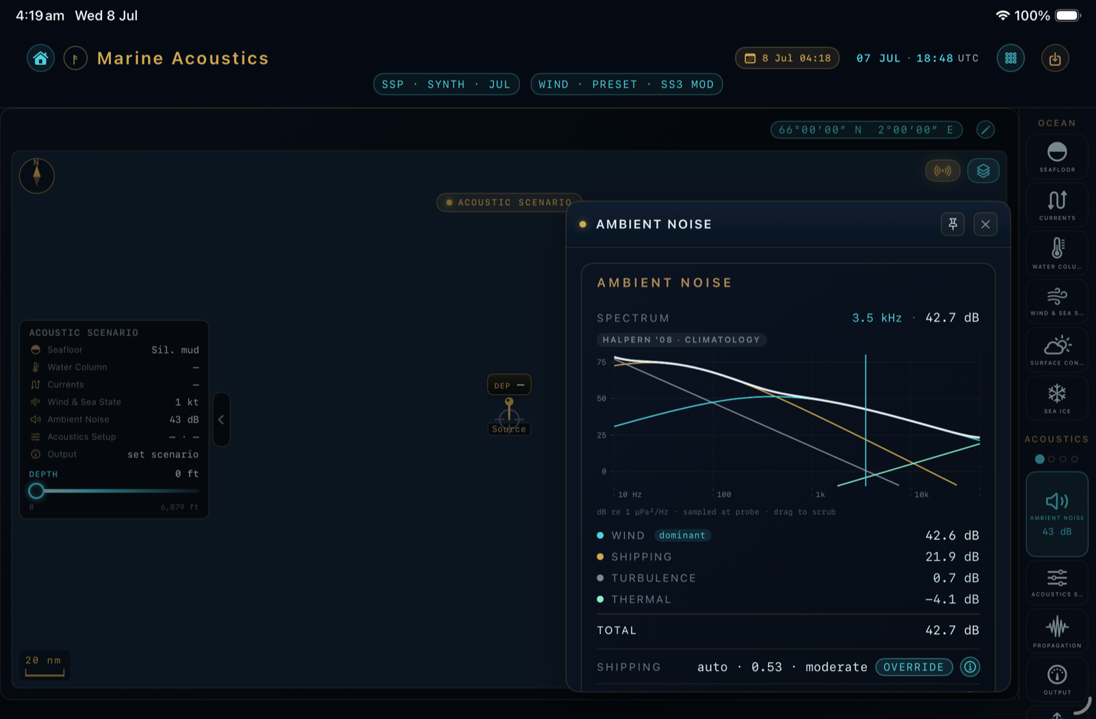
The Ambient Noise panel. The spectrum (here the cursor reads 3.5 kHz · 42.7 dB, sourced from Halpern '08 climatology), then the contributor breakdown — Wind dominant at 42.6 dB, Shipping 21.9, Turbulence 0.7, Thermal −4.1 — summing to the total, with the Shipping row in AUTO (tap OVERRIDE to set it by hand).

The spectrum & frequency cursor
Each noise source is plotted as its own curve, with the power-summed TOTAL drawn brightest on top. A dashed rule marks your working frequency; drag anywhere on the plot to move an inspection cursor and read the total and each contributor at that frequency. The cursor stays where you leave it.
The contributor list
Below the chart, every source is listed at the cursor frequency, loudest first, with the current leader flagged dominant: TURBULENCE, SHIPPING, WIND, THERMAL, OIL RIGS, SNAP SHRIMP, ICE and RAIN, then a TOTAL line. This tells you at a glance which lever is setting the floor.
SHIPPING — auto or override
By default the row reads auto and samples distant merchant-shipping density under the probe (e.g. auto · 0.62 · heavy) — drag the probe across a busy lane and it rises. Tap OVERRIDE to lock a manual value and dial it with a 0–1 slider for sensitivity testing; tap AUTO to hand it back. Bands: light < 0.25, moderate 0.25–0.55, heavy ≥ 0.55.
WIND (NL)
A read-only readout of how much the current wind contributes to the noise floor at your frequency (e.g. 61.2 dB @ 3.5 kHz). Wind speed itself is set on the Wind & Sea State panel; this row shows what that wind actually does to the noise.
OIL RIGS
Noise from offshore platforms within 100 km of the source pin, power-summed into the total. Default INCLUDED; tap to flip to EXCLUDED for a clean-Wenz comparison or when you're far from any installation.

Live vessel traffic LIVE. With MuirWave Live, the shipping curve can switch from the Halpern climatology to an AIS-derived level built from real vessels near you — labelled honestly (AIS-DERIVED · LIVE), never blended, with the difference-vs-climatology shown. A TOP VESSELS block then lists the loudest contributors at 63 Hz; tap one to select it on the map.

§04

Propagation

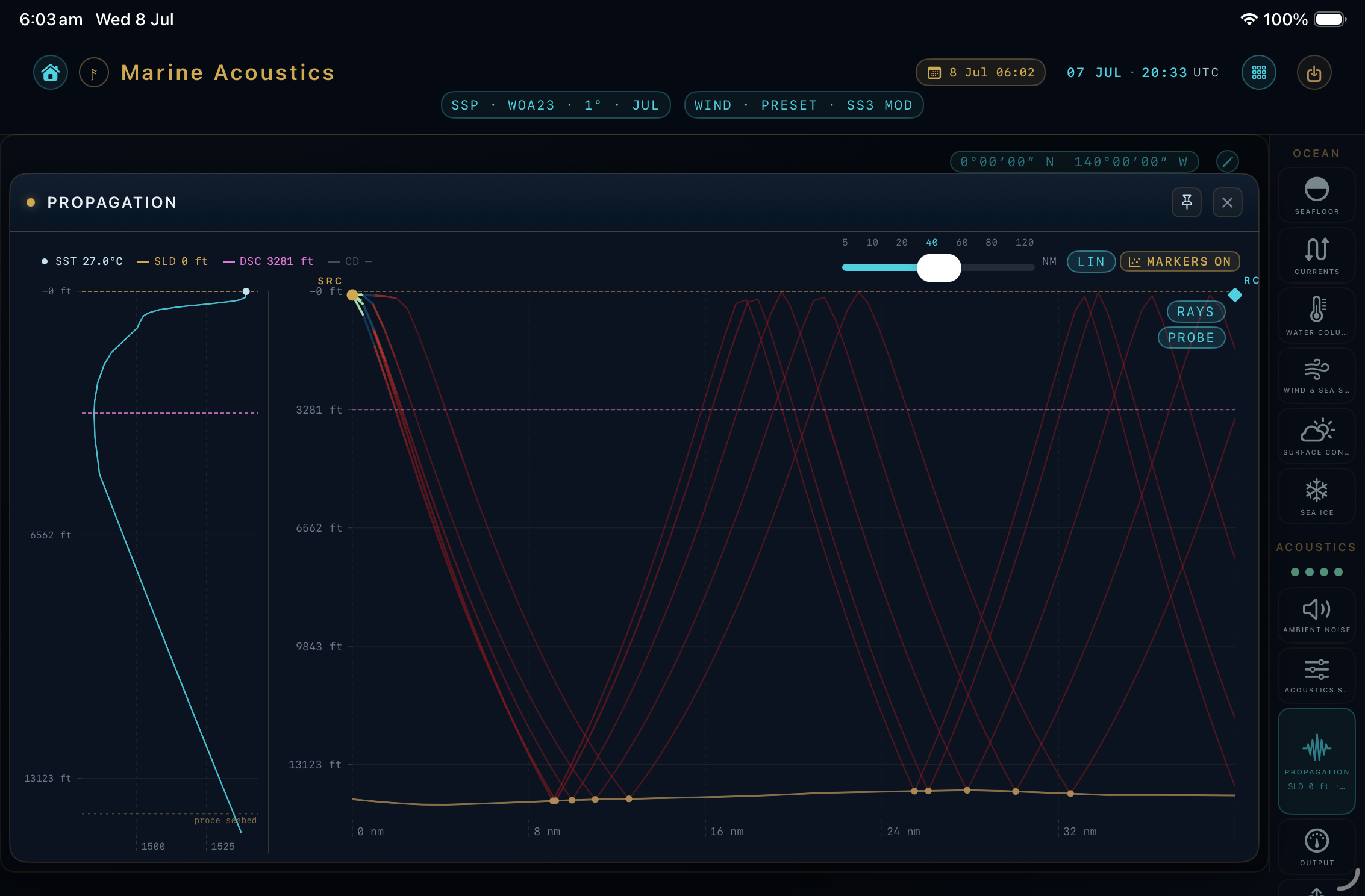
Two charts sharing one depth axis: the sound-speed profile on the left and the ray path on the right. Read a feature on the profile — a channel axis, a duct — and glance straight across to see what the rays do at that same depth. A control strip along the top serves both.

The shared control strip

Legend	The profile readout — SST, SLD, SD, DSC, CD and DE — pinned above both charts so the depth axes line up.
Range slider	Sets the plot's horizontal window: 5 / 10 / 20 / 40 / 60 / 80 / 120 nm (default 40, so the first convergence zone is in view).
LIN / LOG	Depth-axis scale, applied to both charts at once.
MARKERS	Toggles the dashed SLD / DSC / CD reference rules on both the profile and the ray plot.

Left — the sound-speed profile (SVP)

A narrow plot of sound speed versus depth. The shaded band is the surface duct; dashed rules mark the sonic-layer depth, deep sound-channel axis and critical depth. Drag a finger vertically over it to read depth, sound velocity and temperature together at any level (the cursor clears when you lift off). The Depth-Excess (DE) value in the legend is colour-coded to tell you at a glance whether the water is deep enough for reliable convergence-zone propagation:

DE ≥ 300 fa · Green — reliable convergence-zone propagation.

200 – 300 fa · Yellow — marginal.

0 – 200 fa · Grey — positive but too shallow for a dependable CZ.

DE < 0 · Blank — a depth deficit; no number is shown.

Thresholds are always judged in fathoms (1 fa = 1.8288 m), whatever your chosen depth unit.

Right — the ray path

A fan of rays launched from the source, refracting through the profile and reflecting off the surface and seabed. Rays are coloured by their signal excess, and brass dots mark where a ray hits the bottom. Two chips in the corner control what's drawn:

RAYS / FIELD / BOTH	Draw the ray lines, the continuous signal-excess field (a detectability heat wash on a vertical slice), or both. In FIELD or BOTH a detectability key (the signal-excess colour ramp) appears at the bottom-left.
PROBE	Switches the plot into inspection mode: tap or drag anywhere to read the transmission loss and signal excess at that exact range and depth. The chip reads PROBE× while active — tap it to clear.

Drag the markers. The SRC and RCVR pips on the plot are direct handles. Drag SRC up and down to set source depth; drag the RCVR pip anywhere to set its depth and range at once. It's the same as moving the matching sliders on Acoustics Setup, just by hand.

§05

Predicted Output

The scenario as numbers, laid out in the order you'd read the sonar equation — inputs, losses, noise floor, result. Every row updates the instant you nudge any parameter. (Labelled Output on the panel rail, Predicted Output once open.)

Row	What it tells you
SLANT	Straight-line source-to-target distance, in your range unit.
TRANSMISSION LOSS	Loss to the target from the 40-ray beam sum, in dB. Reads a muted — with an OUT OF SOLVER CONE caption when the target sits outside the ray fan.
ABSORPTION α	Seawater absorption at the source depth and frequency, in dB/km.
DUCT CUTOFF	The surface-duct cutoff frequency. Green when your frequency is at or above it (the signal is trapped in the duct), grey when it's leaking. Hidden when there's no surface duct. Related but distinct: DUCT TENDENCY in Surface Conditions is a qualitative verdict on the duct itself; this readout asks whether your frequency is trapped in it.
NOISE LEVEL	The Wenz ambient level, with the dominant contributor tagged.
SEABED BOUNCE	The fan's floor interaction — count, mean grazing angle and mean bottom loss. Reads DIRECT PATH when no ray touches the seabed.
SIGNAL EXCESS	The headline: the signed dB margin after everything is summed. Colour-banded — green (comfortably detectable, SE ≥ +6), yellow (marginal, 0 to +6), orange (just under, −6 to 0), red (not detectable, SE < −6). Zero is the detection threshold.
FOM	Footer summary: the Figure of Merit (how much loss the receiver can afford) and the range at which signal excess falls to zero.

§06

Exporting the scenario

When the picture and the numbers are what you want, the Export action on the panel rail turns the scenario into a document. A picker offers two report styles.

Brief Sheet

A one-glance summary of the scenario, its inputs and its headline results.
Free users can export a watermarked DRAFT Brief Sheet.

Formal EIA Report PRO

A multi-page, regulator-facing PDF documenting inputs, data sources and results for consultancy deliverables.
Part of MuirWave Pro, which also removes the Brief Sheet watermark and unlocks the methodology export.

Tip. The Export action is a rail tile: tap once to reveal it, tap again to open the report picker.