Concepts Explained

All of underwater acoustics is really a single question: a sound starts out at some loudness, weakens as it travels, and competes with background noise — can it still be heard? That balance is the sonar equation, and every panel in MuirWave is one term of it.

MuirWave computes each term from the real ocean at your pin. The rest of this page explains the two that do the heavy lifting: transmission loss (how the sea bends and weakens sound) and the sound-speed profile (why it bends the way it does).

Sound doesn't travel in straight lines underwater. Its speed changes with depth — warmer, shallower water carries sound faster; cold deep water slower; then pressure speeds it up again very deep. Sound rays always bend towards slower water, so this profile shapes where sound goes.

MuirWave builds this profile at your pin from ocean climatology (or live data, with MuirWave Live). It's the single most important input — change the profile and the whole prediction changes. The Water Column panel shows it for any spot.

Models are the best guess available before you sail. Once you're on station with a bathythermograph or a live noise display, you have something better — and MuirWave treats it that way.

Enter a measured layer depth or measured noise points and they outrank every model tier — live feed included — for as long as you keep them switched on. The model keeps running underneath (live data keeps fetching, the comparison curves stay on the plots), so reverting never lands you on stale data, and the gap between model and measurement stays visible: that disagreement is field intelligence, not an error to hide.

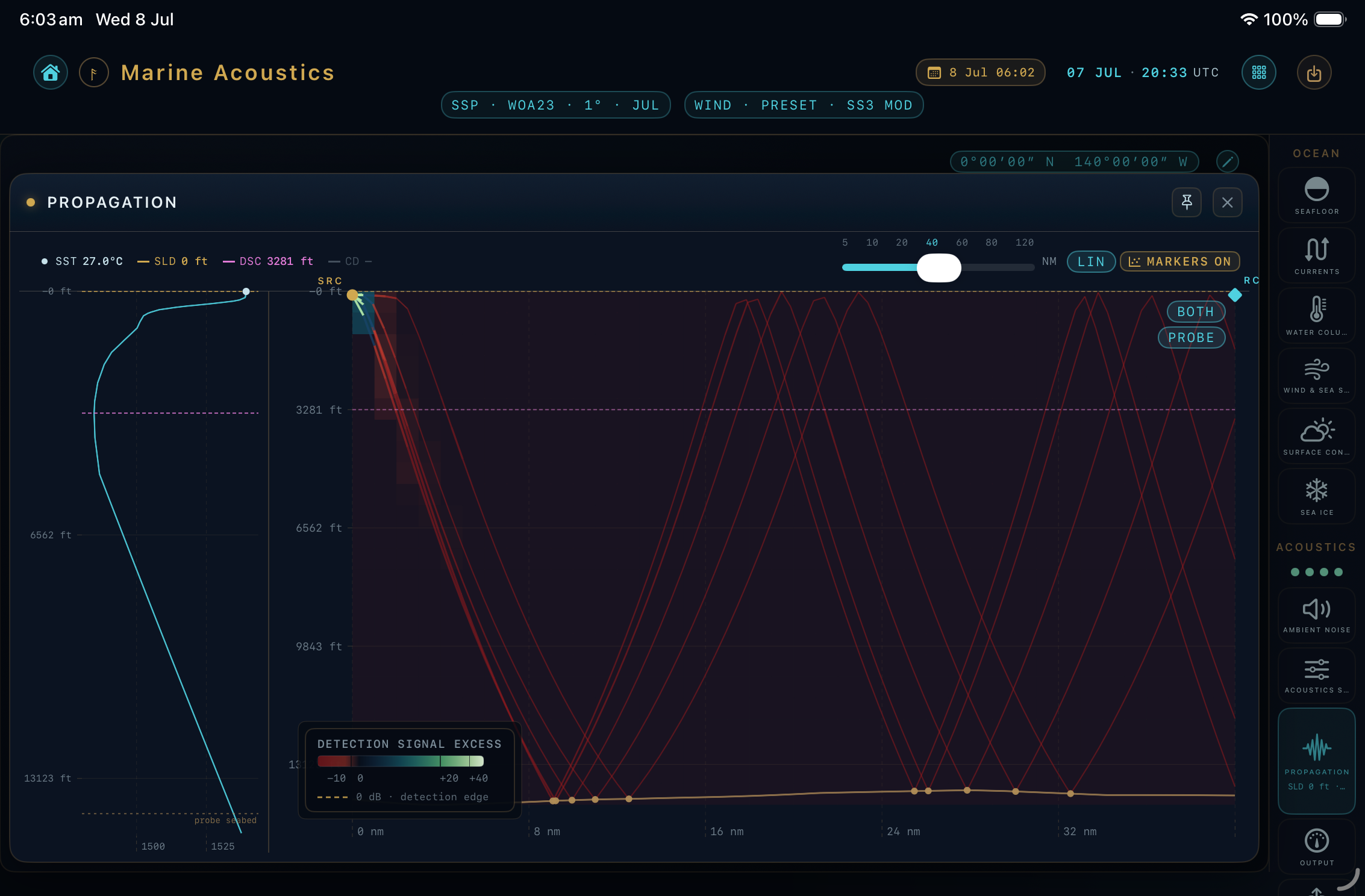
Transmission loss (TL) is simply how much a sound has weakened by the time it reaches a given point — bigger TL means quieter. Because rays bend (§02), sound doesn't fade smoothly: it focuses in some places and thins out in others.

Put the loudness, the loss and the noise together and you get how detectable a source is at each point. MuirWave can paint this across the map as a field — a bird's-eye view of where a source would and wouldn't be heard.

On the Ray Path plot you can switch what's drawn: RAYS shows the ray paths, FIELD shows the continuous detection/loss field, and BOTH overlays them. The structure of the field comes from transmission loss; its overall level comes from the source and receiver you set.

For assessment work, the question flips: instead of "can I hear it?", it's "how far out could this sound affect an animal?" Regulators define thresholds — sound levels above which injury or a behavioural response is expected — that differ by species hearing group and by whether the sound is impulsive or continuous.